4. Tutorial
Before using the full potential of the Capital Analyzer, first some manual configuration must be done. This tutorial shows, which steps need to be performed.
4.1. Demo Configuration
In the directory capital_analyzer/demo_config a fully configured
demo configuration can be found. This example can be used as a template
for the own configuration.
4.2. Preparation
In order to create a custom configuration, it is advisable to create a
complete new directory. In this example, this directory will be called
tutorial. It can be placed everywhere on the hard drive.
Go to the directory capital_analyzer and copy the directory html. Paste
it into the newly created directory tutorial. Your directory should now
look as follow:
- tutorial (dir)
    |- html (dir)
    |   |- bootstrap (dir)
    |   |   |-  <content for bootstrap>
    |   |- index_template.html
    |   |- jquery-3.4.1.min.js
    |   |- main.css
    |   |- main.js
4.3. Prepare Share Data
The first step is to prepare the share data dictionary. This dictionary contains the information, from where to download the share values and also the style and category informations.
For this, in the directory tutorial create a file share_data.py and
paste the following content:
# -*- coding: utf-8 -*-
"""
Module to define the share data.
"""

def get_share_data_dict():
    """
    Returns the dictionary containing the share data.
    """

    share_data_dict = {}

    # fill data here

    return share_data_dict


def get_split_list():
    """
    Returns the data for the share splits.
    """

    split_list = []

    return split_list
Your directory should now look as follow:
- tutorial (dir)
    |- html (dir)
    |   |- bootstrap (dir)
    |   |   |-  <content for bootstrap>
    |   |- index_template.html
    |   |- jquery-3.4.1.min.js
    |   |- main.css
    |   |- main.js
    |- main_downloader.py
    |- share_data.py
The function get_share_data_dict return a dictionary containing the
details of each share (like displayname, color, or download data).
The functio get_split_list will return a list of all splits of shares
to consider. In this tutorial, no splits are considered, hence this function
will not be modified.
In the following, the dictionary share_data_dict will be filled
with details.
4.3.1. Create Dictionary Entry
In the first step, create a dictionary entry for the share. The key
can be chosen arbitrarly, but must be unique. For example, the ISIN, WKN, or
the symbol can be used, as these are unique to each share. In this example,
the WKN (Wertpapierkennnummer) is used. For this example, the details for the
Microsoft share is added. It has the WKN 870747:
share_data_dict["870747"] = {

}
4.3.2. Add Displayname, Color, and Category
The first entries will be the displayname (which will be shown in the legend), the color (which will be used for the lines and bars), and the category (which will be used for the grouping).
share_data_dict["870747"] = {
    "displayname": "Microsoft",
    "color": "b",
    "category": [
        "A"
    ],

}
The displayname can be chosen arbitrarly, here also duplicated to other entries are possible (e.g. for shares that were splitted). For the color, every valid matplotlib color can be entered (see matplotlib documentation). It is also possible to enter a RGB-value-tripple. In this case it is important to enter the values between 0 and 1.
In the field category, the respective categories are listed. A share
can belong to more than one category. The categories are identified
by a unique id, which again can be chosen arbitrarly. For example,
"A", "category_1", "crypto" … can be possible
identifiers. In the example, this share will be in category "A",
which will be a category for a conservative choise.
There exist two already predifined categories. Category "K" is used
to categorize knock outs and other derivatives. Category "X" is used
to categorize the reference indices, to which the personal index is
compared.
Note
An example for a share, that belongs to two categories, could be Knock-Outs.
One might put them in a speculative category with other speculative
assets (e.g. shares from fuel cell or cannabis sector). These shares
should also be categorized into category "K", since in a future
update these derivatives will be evaluated as well.
4.3.3. Add Download Data
For the evaluation, the historical data must be downloaded first. Therefore, the required details must be added.
The data must be downloaded from Ariva.
Note
Wallstreet Online is not supportet at the moment, since it requires an user authetification to download the data.
Ariva:
First, go to https://www.ariva.de/ and open the site of the share. Then go to Kurse –> Historische Kurse and select the stock exchange.
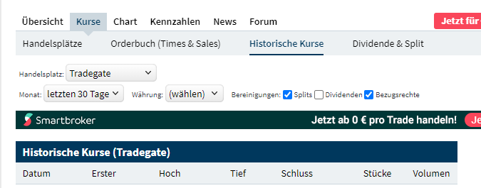
Historical Data of Ariva.
Scroll down to the section “Kurse als CSV-Datei” and click the “Download” button.

Download Historical Data.
Open the Download window of your browser, copy the link of the downloaded file and paste it into a text editor. Here, the fields “secu” and “boerse_id” are important.

Ariva Download Link.
share_data_dict["870747"] = {
    "displayname": "Microsoft",
    "color": "b",
    "category": [
        "A"
    ],
    "download_dict": {
        "data_service": "ariva",
        "download": 1,
        "secu": "415",
        "boerse_id": "131"
    }
}
Note
When e.g. downloading the data for an index, the keys can be different.
For example they might be list and boerse_id. You can insert
them in similar way:
share_data_dict["dowjones"] = {
    "displayname": "Dow Jones",
    "color": "darkorange",
    "category": [
        "X"
    ],
    "download_dict": {
        "data_service": "ariva",
        "download": 1,
        "list": "dow30",
        "boerse_id": "71"
    }
}
This process must be repeated for each share to consider. If you buy a new share, don’t forget to add this share to this dictionary!
Add the following entry for Bitcoin.
share_data_dict["BTC"] = {
    "displayname": "Bitcoin",
    "color": "darkorange",
    "category": [
        "crypto"
    ],
    "download_dict": {
        "data_service": "ariva",
        "download": 1,
        "secu": "111697700",
        "boerse_id": "163"
    }
}
For comparison, the performance of the personal portfolio will be compared
to the performance of the MSCI World. for this, add the following
entry to the dictionary. Category 'X' denotes, that this
entry is used for comparison.
share_data_dict["msci_world"] = {
    "displayname": "MSCI World",
    "color": "lightblue",
    "category": [
        "X"
    ],
    "download_dict": {
        "data_service": "ariva",
        "download": 1,
        "secu" : 226974,
        "boerse_id": "173"
    }
}
4.5. Create File with all Trades and Dividends
In the next step, all trades will be collected into one file. For this,
create a new file trades.py with the following content:
# -*- coding: utf-8 -*-
"""
File containing the list of trades and dividends.
"""
from datetime import datetime
def get_trades():
"""
Returns a list of trades.
"""
list_trades = []
return list_trades
def get_dividends():
"""
Returns a list of dividends.
"""
#dividends
list_dividends = []
return list_dividends
Your directory should now look as follow:
- tutorial (dir)
|- html (dir)
| |- bootstrap (dir)
| | |- <content for bootstrap>
| |- index_template.html
| |- jquery-3.4.1.min.js
| |- main.css
| |- main.js
|- main_downloader.py
|- share_data.py
|- trades.py
The function get_trades will return the list of all trades. The
entries the list are a tuple consisting of the following items:
date of purchase / sell,
identifier of the share,
amount of shares bought /sold,
total amount of money paid (with fees) / obtained (without fees),
fees (optional).
An example entry might look like this:
list_trades.append((datetime(2021, 3, 15), "870747", 0.12470, 25.00, 0.44)) # buy
list_trades.append((datetime(2021, 4, 1), "BTC", 0.00030281, 15.00, 0.00)) # buy
list_trades.append((datetime(2021, 4, 15), "870747", 0.11332, 25.00, 0.44)) # buy
list_trades.append((datetime(2021, 5, 1), "BTC", 0.00031381, 15.00, 0.00)) # buy
list_trades.append((datetime(2021, 5, 17), "870747", 0.12181, 25.00, 0.44)) # buy
list_trades.append((datetime(2021, 6, 1), "BTC", 0.00050002, 15.00, 0.00)) # buy
list_trades.append((datetime(2021, 6, 15), "870747", 0.11515, 25.00, 0.44)) # buy
list_trades.append((datetime(2021, 6, 30), "870747", -0.10000, -22.45, 0.40)) # sell
list_trades.append((datetime(2021, 7, 1), "BTC", 0.00048418, 15.00, 0.00)) # buy
list_trades.append((datetime(2021, 7, 15), "870747", 0.10323, 25.00, 0.44)) # buy
If shares are bought, then the amount of shares, total amount paid, and the fees are all positive. If shares are sold, then the amount of shares and the total amount paid are negative, but the fees are still positive.
In the next step, the dividends must be entered. Here, the same scheme is applied. To maintain consistency of the indices of the tuple, here an amount must be entered as well. For dividends, this amount must be 0. Again, the amount of money obtained must be negative.
list_dividends.append((datetime(2021, 5, 19), "870747", 0.00000, -0.14, 0.02)) #buy
If all trades are inserted, then this file is completed. After each purchase or sell, an entry must be made in this file.
4.6. Create Main File
In the final step, the main file must be created. When running this file,
the analysis is performed and the respective html-file is created.
Therefore, create a new file my_main.py with the following content:
# -*- coding: utf-8 -*-
"""
Main File to run the analysis.
"""
from datetime import datetime
import site
site.addsitedir("../python")
from capital_analyzer.analyze_trades import run_analyze
from trades import get_trades, get_dividends
from share_data import get_share_data_dict
def analyze_trades_demo():
"""
Main function to run the analysis.
"""
if __name__ == "__main__":
analyze_trades_demo()
Your directory should now look like this:
- tutorial (dir)
|- html (dir)
| |- bootstrap (dir)
| | |- <content for bootstrap>
| |- index_template.html
| |- jquery-3.4.1.min.js
| |- main.css
| |- main.js
|- main_downloader.py
|- my_main.py
|- share_data.py
|- trades.py
The configuration is now made in the function analyze_trades_demo.
4.6.1. Basic Parameters
First, some parameters must be defined.
def analyze_trades_demo():
"""
Main function to run the analysis.
"""
# set some configuration files
dir_path_out_html = r"./html"
dir_name_images = "images"
f_name_html = "index.html"
lin_thresh = 3000
currency = "€"
# ...
With dir_path_out_html it is possible to set the path to the directory,
where the html file will be created. Within this directory, a new directory
will be created, where all the images are stored. The name of this
directory can be set with the variable dir_name_images. Finally,
with f_name_html the name of the resulting html-file is defined.
Note
With the parameters dir_name_images and f_name_html it is possible
to have the results of 2 different configurations in one single directory
(for example your portfolio and the portfolio of your parents).
Just select for each configuration a different value for both variables.
With the variable lin_thresh, the symlog scaling of the y-axis can be
adjusted. Until the selected value, a linear scale is used, above this value,
a logarithmic scale is used. Finally, with the variable currency it is
possible to define the currency.
Note
At the moment, it is only possible to have one currency. If you have assets that are only traded in another currency, you must create a new configuration.
4.6.2. Get Data
In the next step, the share data, trades, splits, and dividends are loaded.
# 1. get data
list_trades = get_trades()
list_dividends = get_dividends()
share_data_dict = get_share_data_dict()
split_list = get_split_list()
4.6.3. Grouping for Comparison to Reference Configurations
In the next step, the groups for the comparison to the reference configurations are defined.
#-------------------------------------------------------------------------#
# create a list of all categories to compare
# each entry is a dictionary with the following keys:
# - 'category_list': list of categories to include. Can also be 'all'
# include every share
# - 'displayname': Displayname of the selection
# - 'color: color of the line. Use a matplotlib compatible color
# (see https://matplotlib.org/stable/gallery/color/named_colors.html)
# This list will be used to plot the evolution of each selection (in the
# section 'Capital Estimator')
category_compare_list1 = []
category_compare_list1.append({'category_list': ['A'],
'displayname': "Conservative",
'color': "tab:blue"})
category_compare_list1.append({'category_list': ['crypto'],
'displayname': "Crypto Currencies",
'color': "tab:orange"})
category_compare_list1.append({'category_list': "all",
'displayname': "All",
'color': "tab:green"})
In this tutorial, only one share is considered, both groups will give the same values. But in order to demonstrate the capabilites, both groups are defined.
Note
It is theoretically possible to define any number of groups. But the number of groups should be limited, otherwise the graphs will not be useful.
4.6.4. Grouping for the Personal Index
In the next step, the groups for the personal index are defined. Here, the same fiels are required as above. Furthermore, it is possible to use the same grouping (which is done here).
#-------------------------------------------------------------------------#
# create a list of all categories to compare
# entries are the same as above
# This list will be used to compare an index-based performance. This
# enables a comparison of the performance to the market performance.
# See section 'Personal Index'
category_compare_list2 = category_compare_list1
4.6.5. Define Reference Configurations
In the next step, the reference configurations must be defined. First, the start date and end date of the reference configurations must be defined. The start date can be chosen as the day of the first trade. The end date could e.g. be the expected day of pension.
#-------------------------------------------------------------------------#
# Define some reference configurations to compare your performance
# again a theoretical performance. If you are above the theoretical
# performance, then you can predict your final outcome
# the model of the theoretical evolution is quite simple. Define a
# start capital, a monthly payment and a yearly interest rate. It
# is assumed, that the capital will grow with this interest rate every
# year. If taking an average interest rate (e.g. 7%), this will give
# reasonable results.
start_date_reference_config = datetime(2021, 3, 1)
end_date_reference_config_table = datetime(2062, 2, 17)
Next, the reference configurations must be defined in a list. For each reference configuration, the start capital, the monthly payment, the interest rate, and the start date of the reference configuration must be defined. It is also possible to define different reference configurations with different start dates. Furthermore, a color for the plot must be selected.
reference_config_list = []
reference_config_list.append({
'args': {
'start_capital' : 0,
'monthly_payment' : 25,
'interest' : 1.07,
'start_date' : start_date_reference_config
},
'color': (197 / 255, 90 / 255, 17 / 255)
})
reference_config_list.append({
'args': {
'start_capital' : 0,
'monthly_payment' : 25,
'interest' : 1.10,
'start_date' : start_date_reference_config
},
'color': (244 / 255, 177 / 255, 131 / 255)
})
In this example, two reference configurations were defined. Both have the same start capital of 0 and monthly payment of 25€. In the first case, an interest rate of 7% annually is assumed. In the second case, this interest rate is assumed to be 10%
Now, even more reference configurations can be defined. But for this example, these two configurations should be sufficient.
4.6.7. Create Configuration Dictionary
In this step, the required details are saved in a dictionary and the method to run the analysis is called. This code block can be copied.
#-------------------------------------------------------------------------#
# create configuration dictionary
config = {}
config['share_data_dict'] = share_data_dict
config['list_trades'] = list_trades
config['list_dividends'] = list_dividends
config['split_list'] = split_list
config['dir_path_out_html'] = dir_path_out_html
config['dir_name_images'] = dir_name_images
config['f_name_html'] = f_name_html
config['lin_thresh'] = lin_thresh
config['currency'] = currency
config['category_compare_list1'] = category_compare_list1
config['category_compare_list2'] = category_compare_list2
config['reference_config_list'] = reference_config_list
config['end_date_reference_config_table'] = end_date_reference_config_table
#config['end_date_reference_config_plot'] = end_date_reference_config_plot
config['categories_rel_amount_list'] = categories_rel_amount_list
# 3. analyze data
run_analyze(config)
4.6.8. Run Analysis
In order to run the Analysis, the script my_main.py must be executed.
This will analyze the trades and create the index.html. In this file,
the results can be seen.
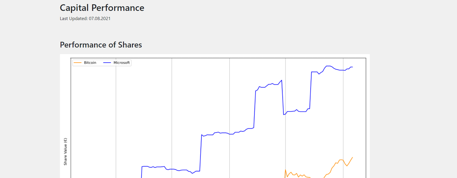
Resulting html-Report.
4.7. Final files
In this section, the resulting files of the tutorial are listed.
4.7.1. main_downloader.py
# -*- coding: utf-8 -*-
"""
Main Downloader module.
"""

from capital_analyzer.download_data import download_data

from share_data import get_share_data_dict


def demo_download_data():
    """
    Method to download the historical share data.
    """

    share_data_dict = get_share_data_dict()

    download_data(share_data_dict)


if __name__ == "__main__":
    demo_download_data()
4.7.2. my_main.py
# -*- coding: utf-8 -*-
"""
Main File to run the analysis.
"""
from datetime import datetime
from capital_analyzer.analyze_trades import run_analyze
from trades import get_trades, get_dividends
from share_data import get_share_data_dict, get_split_list
def analyze_trades_demo():
"""
Main function to run the analysis.
"""
# set some configuration files
dir_path_out_html = r"./html"
dir_name_images = "images"
f_name_html = "index.html"
lin_thresh = 3000
currency = "€"
# 1. get data
list_trades = get_trades()
list_dividends = get_dividends()
share_data_dict = get_share_data_dict()
split_list = get_split_list()
#-------------------------------------------------------------------------#
# create a list of all categories to compare
# each entry is a dictionary with the following keys:
# - 'category_list': list of categories to include. Can also be 'all'
# include every share
# - 'displayname': Displayname of the selection
# - 'color: color of the line. Use a matplotlib compatible color
# (see https://matplotlib.org/stable/gallery/color/named_colors.html)
# This list will be used to plot the evolution of each selection (in the
# section 'Capital Estimator')
category_compare_list1 = []
category_compare_list1.append({'category_list': ['A'],
'displayname': "Conservative",
'color': "tab:blue"})
category_compare_list1.append({'category_list': ['crypto'],
'displayname': "Crypto Currencies",
'color': "tab:orange"})
category_compare_list1.append({'category_list': "all",
'displayname': "All",
'color': "tab:green"})
#-------------------------------------------------------------------------#
# create a list of all categories to compare
# entries are the same as above
# This list will be used to compare an index-based performance. This
# enables a comparison of the performance to the market performance.
# See section 'Personal Index'
category_compare_list2 = category_compare_list1
#-------------------------------------------------------------------------#
# Define some reference configurations to compare your performance
# again a theoretical performance. If you are above the theoretical
# performance, then you can predict your final outcome
# the model of the theoretical evolution is quite simple. Define a
# start capital, a monthly payment and a yearly interest rate. It
# is assumed, that the capital will grow with this interest rate every
# year. If taking an average interest rate (e.g. 7%), this will give
# reasonable results.
start_date_reference_config = datetime(2021, 3, 1)
end_date_reference_config_table = datetime(2062, 2, 17)
reference_config_list = []
reference_config_list.append({
'args': {
'start_capital' : 0,
'monthly_payment' : 25,
'interest' : 1.07,
'start_date' : start_date_reference_config
},
'color': (197 / 255, 90 / 255, 17 / 255)
})
reference_config_list.append({
'args': {
'start_capital' : 0,
'monthly_payment' : 25,
'interest' : 1.10,
'start_date' : start_date_reference_config
},
'color': (244 / 255, 177 / 255, 131 / 255)
})
#-------------------------------------------------------------------------#
# Create a list for the groups of which to compute the realtive amounts.
# has the same structure as above, the key 'color' can be ommited here.
categories_rel_amount_list = category_compare_list1
#-------------------------------------------------------------------------#
# create configuration dictionary
config = {}
config['share_data_dict'] = share_data_dict
config['list_trades'] = list_trades
config['list_dividends'] = list_dividends
config['split_list'] = split_list
config['dir_path_out_html'] = dir_path_out_html
config['dir_name_images'] = dir_name_images
config['f_name_html'] = f_name_html
config['lin_thresh'] = lin_thresh
config['currency'] = currency
config['category_compare_list1'] = category_compare_list1
config['category_compare_list2'] = category_compare_list2
config['reference_config_list'] = reference_config_list
config['end_date_reference_config_table'] = end_date_reference_config_table
#config['end_date_reference_config_plot'] = end_date_reference_config_plot
config['categories_rel_amount_list'] = categories_rel_amount_list
# 3. analyze data
run_analyze(config)
if __name__ == "__main__":
analyze_trades_demo()
4.7.4. trades.py
# -*- coding: utf-8 -*-
"""
File containing the list of trades and dividends.
"""
from datetime import datetime
def get_trades():
"""
Returns a list of trades.
"""
list_trades = []
list_trades.append((datetime(2021,  3,  15), "870747",       0.12470,    25.00,   0.44))  # buy
list_trades.append((datetime(2021,  4,   1),    "BTC",    0.00030281,    15.00,   0.00))  # buy
list_trades.append((datetime(2021,  4,  15), "870747",       0.11332,    25.00,   0.44))  # buy
list_trades.append((datetime(2021,  5,   1),    "BTC",    0.00031381,    15.00,   0.00))  # buy
list_trades.append((datetime(2021,  5,  17), "870747",       0.12181,    25.00,   0.44))  # buy
list_trades.append((datetime(2021,  6,   1),    "BTC",    0.00050002,    15.00,   0.00))  # buy
list_trades.append((datetime(2021,  6,  15), "870747",       0.11515,    25.00,   0.44))  # buy
list_trades.append((datetime(2021,  6,  30), "870747",      -0.10000,   -22.45,   0.40))  # sell
list_trades.append((datetime(2021,  7,   1),    "BTC",    0.00048418,    15.00,   0.00))  # buy
list_trades.append((datetime(2021,  7,  15), "870747",       0.10323,    25.00,   0.44))  # buy
return list_trades
def get_dividends():
"""
Returns a list of dividends.
"""
#dividends
list_dividends = []
return list_dividends
4.8. Next Steps
4.8.1. Look at the demo configuration
The directory demo_config contains a fully configured demonstartion
configuration. This configuration can be the base for you own
configuration.
4.8.2. Create your own configuration
Now it’s up to you: create your own configuration and fill in your trades!
4.8.3. Register Splits
When splits of shares occur, then these must be registered for a correct
evaluation. This is done in the function get_split_list.
Each entry is a tuple with the following items:
old identifier
date of split
split ratio
new identifier
With the old identifier, the prices before the split must be linked. With the new identifier. the prices after the split are linked.